Datapath pipelining

The concept of pipelining extracted from the concept of production lines of vehicles, makes use of breaking down a task into several subtasks and using parallel processing to complete those subtasks. There are two main objectives achieved using pipelining in a digital electronic system.

1. Increasing the throughput of the system.
2. Running the system at higher clock rates.

Increasing the throughput.

If a certain process consists of several sub processes, all those sub processes have to be completed to get the outputs. While one sub process is being carried out, the resources used for other sub processes will be idling. Pipeling reduces these idle times by sending several inputs one after the other without waiting till the first one finishes so that the idling parts of the system processes the next input rather than wasting time.

Running the system at higher clock rates.

Advanced systems running at multi Mega hertz or Giga hertz speeds allow only few nano seconds between clock pulses. (eg: 200MHz system gives only 5ns between clock pulses). This reduces the maximum length and logic allowable for a data path. Through pipelining the critical data paths can be broken down into parts and used by sending the data in several clock cycles without reducing the throughput. Hence the reduction in critical data path lengths can be used to clear timing issues in increasing the system clock rate.

A simple implementation of a pipelined system is shown below.

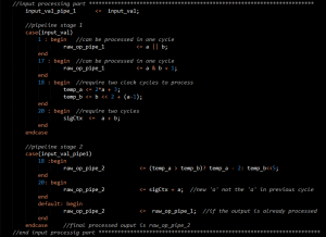
In the above example, the input is processed according to the ‘input_val’. When the ‘input_val’ is 18, intermediate variables are required for the final calculation hence two cycles are required. Although this could have been done in one clock cycle with complex logic that could probably cause timing violations. Therefore the output is processed in the second clock cycle.

In the case of ‘input\val’ 20, a variable which is only available in the next clock cycle is also required. So the output calculation requires two cycles.

If the output can be calculated in one clock cycle, the output is placed in the ‘raw_op_pipe_1’ while that is transferred to the output ‘raw_op_pipe_2’ in each cycle (if the processing didn’t take two cycles). If the processing took two cycles, the output is directly placed in the ‘raw_op_pipe_2’ while the next input is also been processed and written to the ‘raw_op_pipe_1’ in the same clock cycle. Hence the throughput of one output per clock cycle is assured although some inputs require more than one clock cycle for processing. That is the beauty of data path pipelining.