Mathematics of Deep Learning

1 Introduction

Deep learning(DL) is becoming increasingly popular within machine learning community for wide range of applications like speech recognition [1], computer vision [2] and natural language processing [3]. The major advantage in DL is its ability to learn from raw input data. Traditional machine learning techniques require experts in a particular field to design feature extractors using domain knowledge. This requirement hindered the adoption of machine learning in many fields. DL does not suffer from this requirement, hence it is used in many unconventional fields like predicting activity of drug molecules, analyzing particle accelerator data and studying mutations in non-coding DNA on gene expression and disease [4].

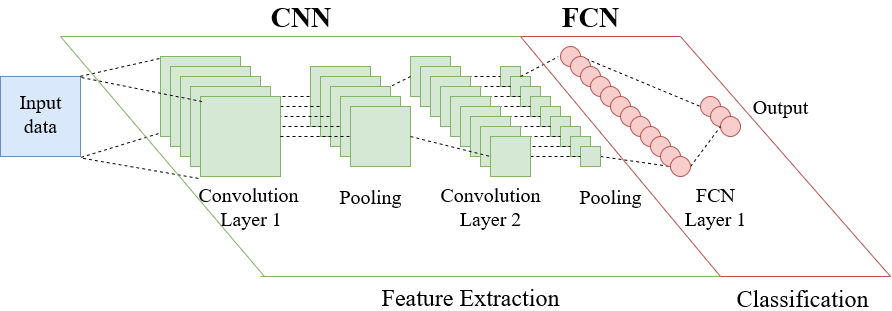
Figure 1: Architecture of Deep Learning Network

Architecture of a deep neural network(DNN) is shown in Fig 1. The DNN consist of two sub networks: convolution neural network(CNN) and fully connected network(FCN). The role of CNN is extracting features in spatially related input data. Multiple convolution layers are used to learn features with hierarchically increasing complexity. For example, if the input data is a raw input image first convolution layer would extract low level features like horizontal and vertical edges. Next convolution layer learns mid level features like motifs created by combination of local edges. Motifs assemble high level features like different parts of objects. Feature extraction is done by applying convolution operator(1) on input data. Rectified linear unit(ReLU) is often used as the activation function for convolution layers. In addition to low computing complexity, ReLu usually learns faster in networks with many layers [4]. Max pooling or mean pooling operation is performed to reduce the input data size. Convolution neural network(CNN) is followed by a fully connected network(FCN) for performing classification. Non-linear functions like sigmoid are preferred as the activation function for FCN. Non-linear activation function maps the input data to a linearly separable space which provides better classification results.

$conv_{x,y} = \sum\limits_{i} w_i.v_i$

DL has shown superior performance compared to other networks. AlexNet [2] was able to achieve top-5 error rate of 17.0% in ImageNet LSVRC-2010 contest outperforming other solutions by a significant margin. DNNs were able to reduce word error rates in speech recognition by 30% over conventional techniques [5]. Although efficiency of DL is seen empirically, the mathematical reasoning for its performance remains elusive [6]. This report presents the mathematical model of DL which is useful in understanding the operation of DL.

2 Preliminaries

2.1 Solving linear systems

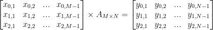
A linear system can be represented by a matrix. The output (y) of the system is given by the multiplication of system matrix (A) and input vector (x). Matrix inversion can be used to find the input when the output and system is known. The problem of interest in DL is finding the system when input and output is known. This problem can be solved using a collection of inputs and outputs. For this lesson we will use the convention of using rows to represent individual inputs and outputs where an element in a row represents a dimension (a feature in ML) of the input/output. The system matrix has the shape of $M\times N$ where M is the number of dimensions in input vector and N is number of dimensions in output vector. If $x0, x1, x3$ are three input vectors and $y0, y1, y3$ are corresponding output vectors, the relationship can be written as (2)

$\begin{bmatrix}x_{0,1} & x_{0,2} & ... & x_{0,{M-1}} \\x_{1,1} & x_{1,2} & ... & x_{1,{M-1}} \\x_{2,1} & x_{2,2} & ... & x_{2,{M-1}}\end{bmatrix}\times A_{M\times N} =\begin{bmatrix}y_{0,1} & y_{0,2} & ... & y_{0,{N-1}} \\y_{1,1} & y_{1,2} & ... & y_{1,{N-1}} \\y_{2,1} & y_{2,2} & ... & y_{2,{N-1}}\end{bmatrix}$

In order to model the system, $M\times N$ parameters need to be determined. One method of solving this problem is multiplying both sides by pseudoinverse of input vectors. The moore-penrose pseudoinverse [7] is defined as (3). A practical way of calculating pseudoinverse is using single value decomposition (SVD) as shown in (4) where U and V are left and right singular-value vectors of A in respective order and D+ is similar to D in SVD of A except non-zero diagonal elements are inversed. However this method is numerically unstable hence small errors in input and output meassurments can create significant errors in calculated model. Therefore different numerical computing mehtods are used to solve the system.

$A^+ = \lim_{\alpha\to 0} (A^T.A + \alpha.I)^{-1}.A^T$

$A^+ = V D^+ U^T$

2.2 Gradient Descent

In order to solve the linear(or nonlinear) system using numerical computing, problem is redefined as an optimization problem. Optimization algorithms iteratively search parameter values that minimize a function output. The function that is being minimized is called objective or loss function. An example of a loss function is the square of Euclidean distance between $y$ and $A.x$ . For linear systems, this loss function is convex which guarantee the convergence. Gradient descent is a numerical computing method used in ML to minimize the loss function. The gradient of the loss function at the minimum is zero and gradient descent algorithm tries to reach this point by iteratively making slow movements towards the direction of gradient. Equation below shows the mathematical form of the algorithm where $\gamma_n$ is the learning rate. In some implementations, learning rate is a function of n which decreases in consecutive steps. Figure 2 shows an illustration of the gradient descent algorihm.

$x_{n+1} = x_n - \gamma_n \nabla F(x_n)$

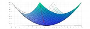
Figure 2: Application of gradient descent algorithm on a loss function

2.3 Back Propagation

Numerical computing methods like gradient descent and its variants require the gradient of a multi dimentional function. This task is accomplished by back propagation algorithm which is an efficient way of computing chain rule of calculus, with a specific order of operation. The chain rule is shown below which can extended to $x \in \mathbb{R}^m$ and $y \in \mathbb{R}^n$ where $\left(\frac{\partial y}{\partial x}\right)$ is the $n \times m$ jacobian matrix

$\frac{\partial z}{\partial x} = \frac{\partial z}{\partial y} \frac{\partial y}{\partial x}$

$\nabla_x z = \left(\frac{\partial y}{\partial x}\right)^T \nabla_y z$

Mathematics of Backpropagation

This explanation is from book chapter : Neural networks and deep learning chapter 2

All methods that are used for training (GDA, SGC) require calculating the gradient of the cost function w.r.t weights and biases. We use the back propagation to make this computation.

The output activation of layer l can be written as follows where sigma is the non-linear activation function

alternatively using weighted input

a^l = \sigma ( z^l )

As a common cost function let’s use quadratic cost function

C = \frac{1}{2n} {\Sigma}_x || y - a^L(x) ||^2

Two assumption are made on the choice of cost function
- The overall cost is the average of the cost for individual inputs
- The cost can be calculated using output activations

The goal of back propagation is calculating following entities

\frac{\delta C}{\delta w_{jk}^l} \qquad \frac{\delta C}{\delta b_{j}^l}

To achieve the goal let’s first calculate an intermediate term: Change of cost w.r.t weighted input

Gradient of the cost function w.r.t activation for the output layer(L) (assuming quadratic cost function take the derivative w.r.t activation a) and hidden layers can be written as

By putting everything together we can write the partial derivative of the cost function as follows. Here to obtain the value w.r.t to biases and weights from the respective delta value we use the simple chain rule

2.4 Bernoulli and Multinoulli Distribution

Deep learning is widely used for object classification. A neural network that classifies input to $N$ different classes produce an output vector $y \in \{0,1\}^n$ . Consider the simple case of $N = 1$ , then the probability distribution of the network output should follow a bernoulli distribution. A generalized version of bernoulli distribution is introduced in [8] called multinoulli distribution. Probability mass function of multinoulli distribution is given by (8)

$Mu(x|1,\theta) = \prod_{j=1}^{N} \theta^{\prod x_j = 1}$

3 Mathematical Model of Deep Learning

3.1 Inference Model

The mathematical model for inference in a DNN can be written as below where $W^n$ represents the weight matrix at $n^{th}$ layer and $\psi_n$ represent the elementwise nonlinear activation function used in $n^{th}$ layer. In DNN, convolution layers ( $\psi_{1,2,...}$ ) generally use Rectified Linear Unit(ReLu) activation and fully connected layers ( $\psi_k$ ) use softmax activation since output of convolution layers are in $\left[0,\infty\right)$ and softmax maps this domain to $\left[0,1\right)$ .

$\Phi (X,W^1,W^2,...,W^k) = \psi_k(\psi_{k-1}(...\psi_2(\psi_1(X.W^1).W^2)...W^{k-1})W^k)$

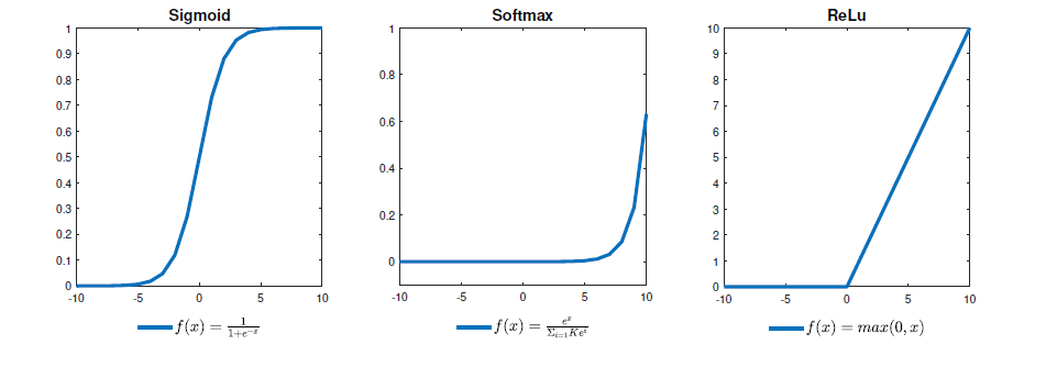
Figure 3: Widely used activation functions

The hierarchical structure of DNN is made possible by the use of non-linear activation function. If activation function is not present all layers can be replaced by a single layer. In the first generation neural networks (perceptrons), threshold function is used as the activation function. It has been shown that perceptron is a universal digital function approximator. The second generation neural networks prefer sigmoid activation function because they can approximate any continuous function. However sigmoid activation has low learning performance because the gradient decay to zero quickly. The modern DNN widely use ReLu for convolution layers and Softmax for fully connected layers.

3.2 Training Model

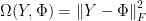
Training of neural networks refer to finding the optimum weight parameters. However learning algorithms differ from optimizing algorithms because the primary goal of learning is to predict the output for unseen data which require avoiding overfitting to training data. Below equation shows the mathematical representation of learning problem. According to our convention each row of $X \in \mathbb{R}^{N \times D}$ represent a single $D$ dimensional input and each row of $Y \in\left\{0,1\right\}^{N\times C}$ represent the membership of one of the C classes.

$min_{W^k} \big\{ \Omega\left(Y,\Phi\left(X,W^1,...,W^K\right)\right) + \lambda\Theta(W^1,...,W^K) \big\}$

$\Omega(Y,\Phi) = \left\lVert Y - \Phi \right\rVert_F^2$

$\Theta(W) = \Sigma_{k=1}^{K} \left\lVert W^k \right\rVert_F^2 \; where \; \lambda > 0$

In the above equation, $\Omega(Y,\Phi)$ is a loss function that measure the agreement between the true output and the predicted output. $\Theta$ is a regularization function that prevents overfitting. $\lambda$ is used as a balancing parameter.

In order to minimize loss function numerical computing methods like gradient descend algorithm is used. However most learning algorithms are typically guarantee to converge to a critical point. Figure below shows different critical points present in non convex functions. Although there is no rigorous proof, experimental results suggests that when network size is large enough and ReLu activation is used all local minima could be global [7].

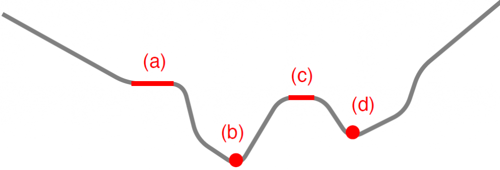
(a) saddle point, (b) global minima, (c) plateau, (d) local minima

4 Summary

This report discusses the mathematical aspect of deep learning as an attempt to understand its superior performance. Deep learning does not depend on input or output data types hence the technique can be applied in many fields. Recent advancements in deep learning have introduced several techniques to improve the performance of generic implementation. Techniques like pooling has improved the numerical stability of the system. The introduction or ReLu activation function has resolved the local minima problem because of the global optimality in positive homogenous networks. The development of hardware and optimization has accelerated adoption of deep learning. With continuous success in variety of fields, deep learning is becoming a dominating technology in future applications.